Examples¶

Real- and Imaginary-Time Evolution with McLachlan’s Principle¶

This example runs two separate evolutions of an 8-qubit transverse-field Ising chain

\[H = -J \sum_i Z_i Z_{i+1} - h \sum_i X_i .\]

For \(h < J\) the ground state is ferromagnetically ordered along \(Z\), for \(h > J\) it is a paramagnet polarized along \(X\), and \(h = J\) is the quantum critical point.

	Real time (VarQRTE)	Imaginary time (VarQITE)
Evolution	\(\|\psi(t)\rangle = e^{-iHt}\|\psi_0\rangle\)	\(\|\psi(\tau)\rangle \propto e^{-H\tau}\|\psi_0\rangle\)
What it is for	Dynamics: what an experiment would see after a quench	Cooling: excited states decay as \(e^{-(E_k-E_0)\tau}\), leaving the ground state
`extract_gradient`	`which="real_time"`	`which="imag_time"`
In this example	\(J = 0.25,\ h = 1\), start \(\|0\ldots0\rangle\), plot \(m_z(t)\)	\(J = h = 1\), start \(\|+\ldots+\rangle\), plot \(E(\tau)\), \(\mathrm{Var}[H](\tau)\)

In both cases, McLachlan’s variational principle turns the evolution into the linear system \(\mathrm{Re}(G)\,\dot\theta = b\) at every step. Only \(b\) depends on the direction. BowtieQGT provides \(G\) and \(b\), and scipy.integrate.solve_ivp integrates \(\dot\theta\). A small regularization \(\lambda I\) takes care of the redundant directions of \(G\).

1. Real time: magnetization after a quench¶

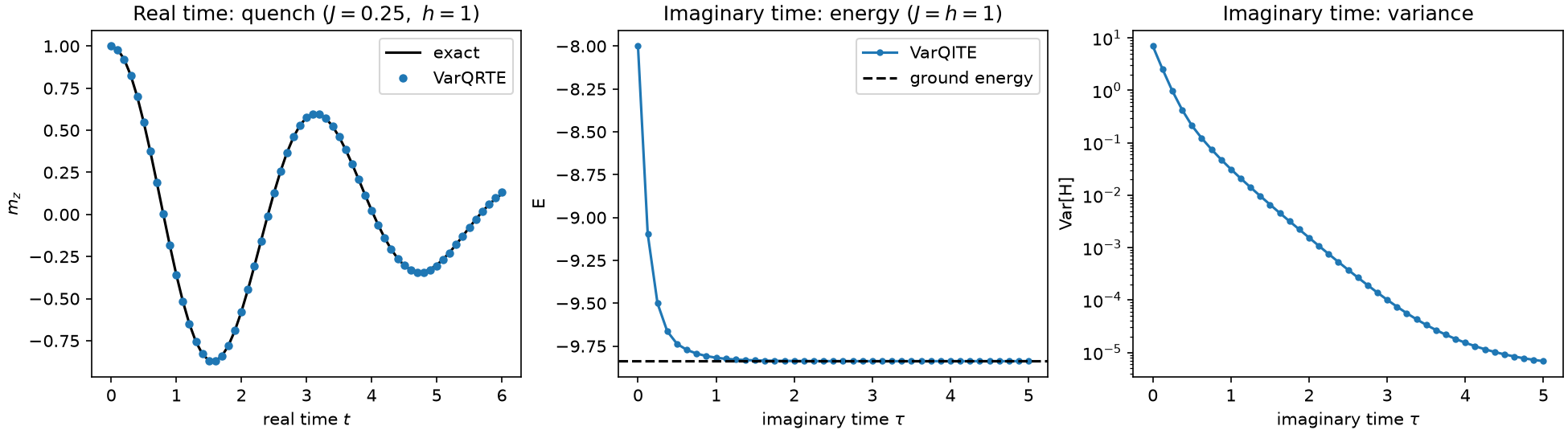
Starting from \(|0\ldots0\rangle\) (all spins along \(+Z\)), the strong field makes every spin precess about \(X\), so the magnetization \(m_z = \langle\sum_i Z_i\rangle / n\) swings from \(+1\) down to about \(-0.9\) and back, with period \(\sim\pi/h\). The weak \(ZZ\) coupling spreads correlations along the chain and dephases the precession, so the oscillations shrink and lose their regularity. VarQRTE follows the exact curve over the whole window (left panel).

2. Imaginary time: ground state at the critical point¶

Starting from \(|+\ldots+\rangle\), the ground state at \(h \to \infty\), the energy decreases monotonically to the exact critical ground energy (middle panel). The variance \(\mathrm{Var}[H]\) falls by six orders of magnitude (right panel), which certifies that the state is an eigenstate and not just a low-energy state. Imaginary time \(\tau\) has no physical meaning here; it only measures how far the cooling has progressed.

Choice of ansatz¶

n_local with rx/ry rotations and rzz bricks is a Trotter circuit with free angles. It contains \(e^{-iHt}\) at short times, and its light cones stay narrow, which is what makes the bowtie method cheap. Hardware-efficient ansätze with fixed CNOT chains, such as efficient_su2, spread every light cone over the whole chain and track this quench much less accurately (error above 0.05 from \(t \approx 3\) with 3 repetitions). With their default ry/rz gates they cannot start the quench at all: at \(\theta = 0\) the required direction \(-iX|0\rangle\) is outside the ansatz.

Left: real-time magnetization after a quench, VarQRTE vs exact. Middle and right: imaginary-time energy and variance of VarQITE.

The script runs in about seven minutes on a laptop. It needs matplotlib and scipy. It is also in the repository as docs/examples/mclachlan_ising.py.

import matplotlib.pyplot as plt
import numpy as np
from qiskit import QuantumCircuit
from qiskit.circuit.library import n_local
from qiskit.quantum_info import SparsePauliOp, Statevector
from scipy.integrate import solve_ivp
from scipy.sparse.linalg import eigsh, expm_multiply

from bowtie_qgt.bowtieqgt import BowtieQGT

n = 8


def ising(J: float, h: float) -> SparsePauliOp:
    """Open-chain transverse-field Ising Hamiltonian."""
    return SparsePauliOp.from_sparse_list(
        [("ZZ", [i, i + 1], -J) for i in range(n - 1)] + [("X", [i], -h) for i in range(n)],
        num_qubits=n,
    )


def brickwork(reps: int) -> QuantumCircuit:
    """rx/ry layers and rzz bricks. All angles zero prepares |0...0⟩."""
    return n_local(n, ["rx", "ry"], "rzz", entanglement="pairwise", reps=reps)


def mclachlan_rhs(bowtie: BowtieQGT, which: str, regularization: float = 1e-6):
    """θ̇ = (Re G + λ I)^{-1} b, with b for which="real_time" or "imag_time".

    The small λ handles the redundant directions of G.
    """

    def rhs(_t, theta):
        generalized_qgt, _ = bowtie.evaluate(theta)
        qgt = bowtie.extract_qgt(generalized_qgt)  # real part, as McLachlan requires
        b = bowtie.extract_gradient(generalized_qgt, which=which)
        return np.linalg.solve(qgt + regularization * np.eye(len(b)), b)

    return rhs


def evolve(bowtie: BowtieQGT, which: str, times: np.ndarray) -> np.ndarray:
    """Integrate McLachlan's equation from θ = 0; returns θ at each time, shape (T, N)."""
    solution = solve_ivp(
        mclachlan_rhs(bowtie, which),
        (times[0], times[-1]),
        np.zeros(bowtie.qc.num_parameters),
        t_eval=times,
        rtol=1e-6,
        atol=1e-8,
    )
    return solution.y.T


# ======================================================================================
# 1. REAL-TIME evolution (VarQRTE): |ψ(t)⟩ = e^{-iHt}|0...0⟩
#    Magnetization oscillations after a quench.
# ======================================================================================
hamiltonian = ising(J=0.25, h=1.0)
magnetization = SparsePauliOp.from_sparse_list([("Z", [i], 1 / n) for i in range(n)], n)
ansatz = brickwork(reps=3)
times = np.linspace(0, 6, 61)  # real time t
thetas = evolve(BowtieQGT(ansatz, hamiltonian), "real_time", times)
m_varqrte = [
    Statevector(ansatz.assign_parameters(theta)).expectation_value(magnetization).real
    for theta in thetas
]
# Exact reference: exp(-iHt)|0...0⟩ on the full 2^n state vector.
psi0 = np.zeros(2**n, dtype=complex)
psi0[0] = 1
exact_states = expm_multiply(
    -1j * hamiltonian.to_matrix(sparse=True), psi0, start=times[0], stop=times[-1], num=len(times)
)
m_exact = [Statevector(psi).expectation_value(magnetization).real for psi in exact_states]
print(f"Real time:      max |m_z - exact| = {np.max(np.abs(np.subtract(m_varqrte, m_exact))):.1e}")

# ======================================================================================
# 2. IMAGINARY-TIME evolution (VarQITE): |ψ(τ)⟩ ∝ e^{-Hτ}|+...+⟩
#    Ground-state preparation at the critical point.
# ======================================================================================
hamiltonian = ising(J=1.0, h=1.0)
ansatz = QuantumCircuit(n)
ansatz.h(range(n))  # θ = 0 now prepares |+...+⟩
ansatz.compose(brickwork(reps=4), inplace=True)
bowtie = BowtieQGT(ansatz, hamiltonian)
taus = np.linspace(0, 5, 41)  # imaginary time τ
energies, variances = [], []
for theta in evolve(bowtie, "imag_time", taus):
    generalized_qgt, energy = bowtie.evaluate(theta)
    energies.append(energy)
    variances.append(bowtie.extract_variance(generalized_qgt))
ground_energy = eigsh(hamiltonian.to_matrix(sparse=True), k=1, which="SA")[0][0]
print(f"Imaginary time: E = {energies[-1]:.5f}, exact {ground_energy:.5f}")
print(f"                Var[H] = {variances[-1]:.1e}")

# --- Plots ----------------------------------------------------------------------------
fig, (ax_rt, ax_e, ax_var) = plt.subplots(1, 3, figsize=(13, 3.6), layout="constrained")
ax_rt.plot(times, m_exact, "k-", label="exact")
ax_rt.plot(times, m_varqrte, "o", ms=4, label="VarQRTE")
ax_rt.set(xlabel="real time $t$", ylabel=r"$m_z$", title=r"Real time: quench ($J=0.25,\ h=1$)")
ax_rt.legend()
ax_e.plot(taus, energies, "o-", ms=3, label="VarQITE")
ax_e.axhline(ground_energy, color="k", ls="--", label="ground energy")
ax_e.set(xlabel=r"imaginary time $\tau$", ylabel="E", title=r"Imaginary time: energy ($J=h=1$)")
ax_e.legend()
ax_var.semilogy(taus, variances, "o-", ms=3)
ax_var.set(xlabel=r"imaginary time $\tau$", ylabel="Var[H]", title="Imaginary time: variance")
fig.savefig("mclachlan_ising.png", dpi=150)

Examples¶

Real- and Imaginary-Time Evolution with McLachlan’s Principle¶

1. Real time: magnetization after a quench¶

2. Imaginary time: ground state at the critical point¶

Choice of ansatz¶

See Also¶